On-the-fly rendering¶

Relevant headers

framework/parameters/render.cpp
framework/domain/io/init.cpp
framework/domain/io/render.cpp
output/render/renderer.h
output/render/renderer.cpp
output/render/raymarch.hpp
output/render/fieldlines.h
output/render/slice2d.hpp
output/render/transfer_fn.h
output/render/composite.h
output/render/axes.h
output/render/colorbar.h
output/render/png.h
output/render/reduce.hpp
scripts/render.py

1.5.0

Entity can render scalar fields directly to .png images on the GPU during the run. At every output cadence the renderer prepares a scalar field, integrates it on the device, composites the result across all MPI ranks, and writes a finished image to <simulation.name>/renders/. No field data is written to storage, and the output is seamless across MPI domain boundaries -- there are no visible seams where subdomains meet.

The feature is metric- and engine-aware: it picks a rendering mode automatically from the simulation dimension and coordinate system.

Simulation	Mode	What is drawn
3D Minkowski (Cartesian)	volume ray-march	a translucent volume render of the scalar
2D Minkowski (Cartesian)	flat slice	the `(x, y)` plane as an opaque heatmap
2D Spherical / QSpherical (SRPIC)	meridional slice	the `(r, θ)` half-plane mapped to Cartesian
2D Kerr–Schild / QKerr–Schild (GRPIC)	meridional slice	same, with GR moments
1D, or 3D non-Cartesian	--	no-op

Where the work lives

The renderer is split like the Writer: a non-templated out::Renderer owns all metric-agnostic, host-side work (config parsing, cadence, the MPI composite, PNG encoding), while the templated Metadomain<S, M>::Render owns the per-(engine, metric, dimension) field preparation and the device kernel launch. The same ComputeMoments / FieldsToPhys code paths used by the field output are reused, so renders are consistent with the ADIOS dumps.

Enabling the renderer¶

The renderer is configured in its own top-level [render] table (independent of [output]), with no additional compile-time flags required.

[render]
  # Toggle for the renderer
  #   @type: bool
  #   @default: false
  enable = true
  # Number of timesteps between renders
  #   @type: uint
  #   @default: 0
  #   @note: when 0, `interval_time` is used instead
  interval = 0
  # Physical (code) time between renders
  #   @type: float
  #   @default: -1.0
  #   @note: when < 0, the cadence is controlled by `interval`
  interval_time = 1.0
  # Output image size in pixels (the rendered region; the PNG is wider if a
  # colorbar margin is added, see `colorbar_outside`)
  #   @type: int [> 0]
  #   @default: 1024
  width  = 1024
  height = 1024
  # Convenience: force a square frame (width == height == resolution), e.g.
  # for a dome master. Overrides `width`/`height` when > 0
  #   @type: int [> 0]
  #   @default: 0 (use width/height)
  resolution = 0

The cadence works like the regular field output: set either a step interval or a physical interval_time. If neither is set, the renderer falls back to output.interval / output.interval_time.

Scenes and quantities¶

Each rendered field is a scene -- one [[render.scene]] table maps to one stream of PNGs (e.g. N_00000001.png, N_00000002.png, ...). Repeat the table to render several quantities at once.

[[render.scene]]
  # Scalar field to render (see the grammar below)
  #   @required
  #   @type: string
  field    = "N"
  # PNG filename prefix; files are `<prefix><cycle>.png`
  #   @type: string
  #   @default: "<field>_"
  prefix   = "N_"
  # Colorbar title
  #   @type: string
  #   @default: "<field>"
  label    = "N / n0"
  # Transfer-function value range
  #   @type: float
  min      = 0.1
  max      = 100.0
  # Map the value range logarithmically (requires min > 0)
  #   @type: bool
  #   @default: false
  log      = true
  # Colormap name
  #   @type: string
  #   @default: "viridis"
  #   @enum: "viridis", "inferno", "plasma", "cool2warm", "gray", "RdBu_r" plus
  #          the CMasher maps: "dusk", "cosmic", "freeze", "apple", "gothic",
  #          "sunburst", "voltage", "ocean", "fusion", "prinsenvlag"
  colormap = "viridis"

Field grammar¶

A render needs a scalar, so vector quantities are given as a magnitude or a single component. The field string is parsed as follows:

`field`	Meaning
`N`, `Nppc`, `Rho`, `Charge`	scalar particle moments (number, per-cell count, mass & charge density)
`T{i}{j}`	one stress–energy component; `i,j` ∈ `{t,x,y,z}` or `{0,1,2,3}` (e.g. `Txx`, `Ttt`, `T0x`)
`V{i}`	one bulk-velocity component; `i` ∈ `{x,y,z}` or `{1,2,3}`
`Vmag`	bulk-speed magnitude \(\sqrt{V_1^2 + V_2^2 + V_3^2}\)
`{E,B,J}mag`	field-vector magnitude \(\lvert\cdot\rvert\)
`{E,B,J}{1,2,3}` or `{E,B,J}{x,y,z}`	one (signed) physical field component

Moments accept a per-species suffix _<id>: e.g. N_1 (species 1 only), Rho_2, Txy_1_2 (species 1 & 2), V1_3. With no suffix the moment sums over all massive species. An invalid species id logs a warning and skips that scene rather than aborting the run.

Engine differences

Moments follow the engine, exactly as in the field writer:

SRPIC -- V is the tetrad-basis bulk 3-velocity (normalized by Rho); T is the tetrad-basis stress–energy.
GRPIC -- V is the Eckart-frame 4-velocity, so Vt/V0 (\(= u^0 = \Gamma/\alpha\)) is also a valid component; T is contravariant. The E field slot holds the electric displacement \(\bm{D}\), so Emag renders \(\lvert\bm{D}\rvert\).

A bare vector (E, B, J) is not renderable -- pick a component or a magnitude.

Transfer function¶

Each scene maps the scalar through a transfer function: the colormap colors the value, and (in 3D volume mode) a piecewise-linear opacity ramp sets how much each sample contributes. In 2D slice mode each pixel is a single opaque sample, so the opacity ramp is ignored and the colormap is drawn at full opacity.

Colormaps

Besides the built-in viridis, inferno, plasma, cool2warm, gray, and RdBu_r (the reversed ColorBrewer red-blue diverging map, as in matplotlib), ten perceptually-uniform maps from CMasher are bundled: the sequential dusk, cosmic, freeze, apple, gothic, sunburst, voltage, ocean, and the diverging fusion, prinsenvlag. Any of these names (with an optional cmr. prefix for the CMasher maps) can be used anywhere a colormap is accepted -- scene volumes, 2D slices, field-line tubes/contours, and the colorbar. The CMasher maps are stored as 33-anchor downsamplings of the published tables (error < 0.02, visually indistinguishable) and re-implemented from the CMasher source under its BSD-3-Clause license (© 2019-2021 Ellert van der Velden); RdBu_r is from ColorBrewer (© Cynthia A. Brewer, Apache-2.0).

render colormaps

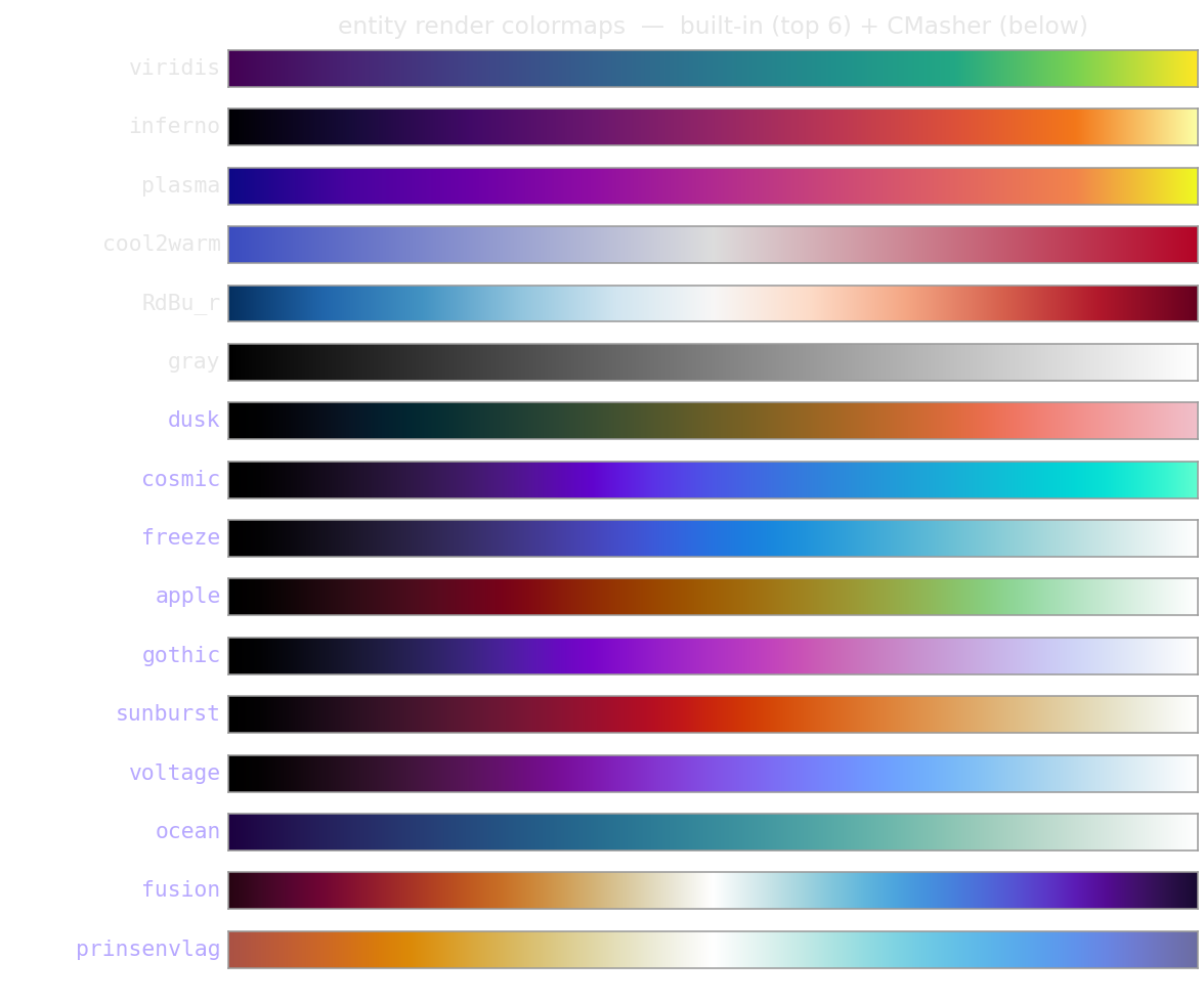
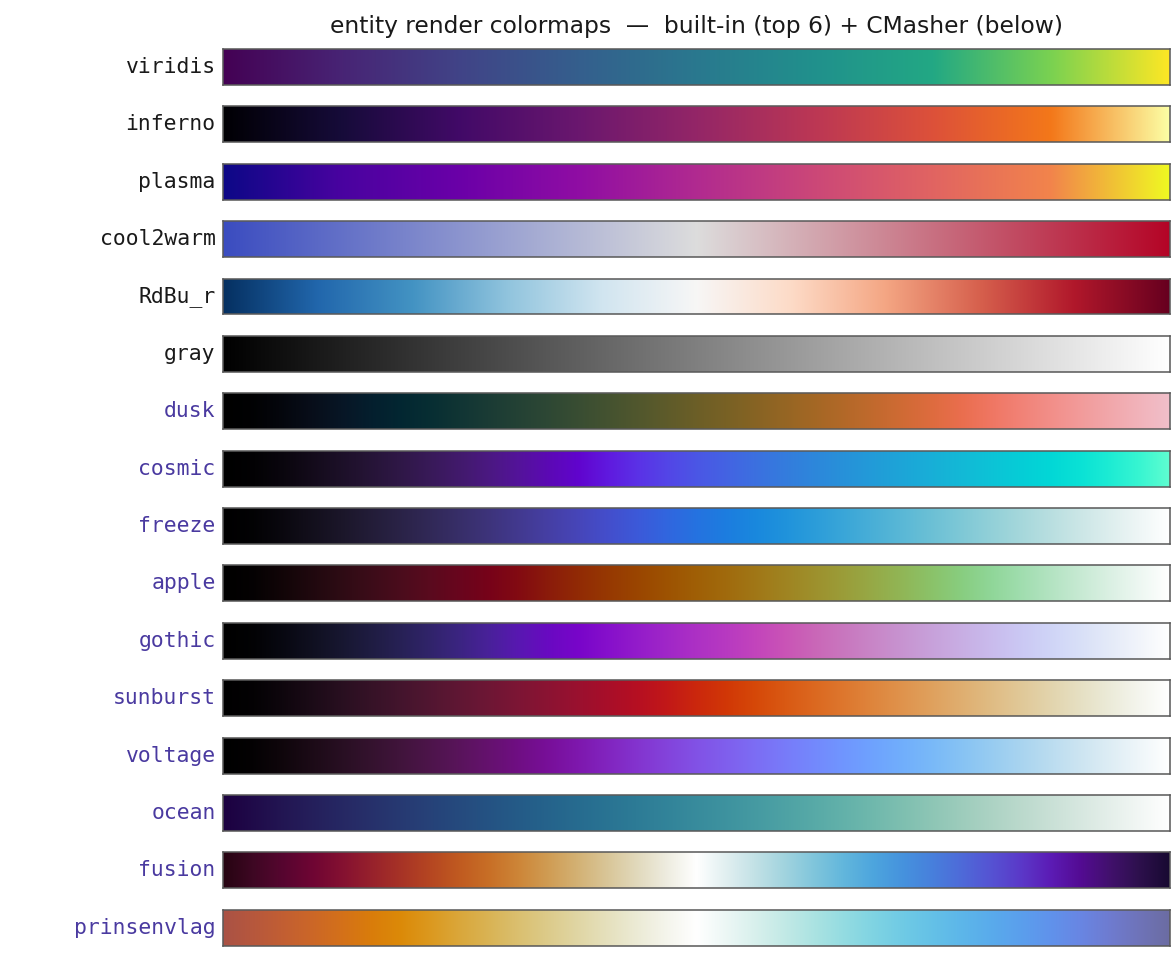
The colormaps accepted by colormap = "...": the six built-ins on top, the ten bundled CMasher maps below (cool2warm, RdBu_r, fusion, and prinsenvlag are diverging). Swatches are rendered from the exact anchor tables shipped in transfer_fn.h.

[[render.scene]]
  # ...
  # Opacity control points [position in 0..1, alpha in 0..1] (3D volume only)
  #   @type: array<array<float>>
  #   @note: signed components pair well with a symmetric min/max and "cool2warm"
  alpha = [[0.0, 0.0], [0.2, 0.15], [1.0, 0.6]]
  # Explicit colorbar tick values (optional; default = 5 evenly spaced)
  #   @type: array<float>
  colorbar_ticks = [0.1, 1.0, 10.0, 100.0]

Top-level options control the overall appearance:

[render]
  # Opaque background RGB (0..1) shown through transparent / low-opacity pixels
  #   @type: array<float> [size 3]
  #   @default: [0.0, 0.0, 0.0]
  background       = [0.0, 0.0, 0.0]
  # Draw a colorbar (gradient + ticks + label) on each PNG
  #   @type: bool
  #   @default: true
  colorbar         = true
  # Put the colorbar in an added right margin instead of overlaying the data
  #   @type: bool
  #   @default: true
  colorbar_outside = true
  # Number of color/opacity LUT entries
  #   @type: int [> 1]
  #   @default: 256
  n_lut            = 256

Render region¶

By default the renderer covers the whole domain. An axis-aligned sub-region can be selected in the [render.extent] table with x1 / x2 / x3 (physical/world coordinates, one [lo, hi] pair per axis). Any axis left unset spans the full extent, and the limits are clamped to the domain.

[render.extent]
  # Render region [lo, hi] along each axis, in physical/world coordinates
  #   @type: array<float> [size 2]
  #   @default: [] (full extent)
  x1 = [-64.0, 64.0]   # crop x1 to this range
  x3 = [0.0, 128.0]    # crop x3; x2 spans the full extent

The behavior follows the mode:

3D volume — the volume is depth-clipped to the box (each domain's march AABB is intersected with the region; domains fully outside are skipped), the wireframe spine and axes frame the region, and the default camera zooms to it. samples then spans the region diagonal, so the effective sampling density increases as you crop in. Field-line tubes clip to the region automatically.
2D slice — the slice window is framed to the region. For a spherical / Kerr--Schild slice, x1 crops the radius r and x2 the polar angle theta, and the meridional window is the bounding box of that cropped wedge.

Cropping is a view operation: the seamless multi-domain composite and the field-line coarse field are unaffected (the field lines are still traced over the full field, then clipped to what's visible).

Moving view (tracking a feature)¶

The region can translate over time to keep a propagating feature in frame (e.g. a shock). This is configured in [render.moving_view]: velocity is a world-units-per-sim-time vector; the region (and, in 3D, the camera — a pure pan, so the view direction and zoom are fixed) shifts by velocity * max(0, t - start_time). The start_time delay lets an initial ramp-up finish before the view starts moving.

[render.extent]
  x1 = [0.0, 512.0]      # initial window (a slab of the domain)

[render.moving_view]
  # Velocity of the moving view in world units
  #   @type: array<float> [size 2 or 3]
  #   @default: [] (static view)
  velocity   = [0.9, 0.0]  # pan along +x1 at 0.9 c ...
  # Sim time at which the view starts moving (static before it)
  #   @type: float
  #   @default: 0.0
  start_time = 200.0       # ... starting at t = 200

The window keeps its size and slides; all ranks advance the view with the same frame time, so the composite stays seamless. Pair it with [render.extent] — without a region the window would just pan off the full domain.

Volume rendering (3D)¶

For 3D Minkowski runs each pixel casts a ray and integrates the transfer function front-to-back with premultiplied "over" compositing. Sampling is global: every rank marches at the same world-space positions \(t_k = k\,\mathrm{d}s\) from the shared camera, with a step \(\mathrm{d}s\) identical on all ranks. Each global sample therefore lands in exactly one subdomain, so the ordered cross-domain composite reproduces the single full-ray integral exactly.

[render.volume]
  # Number of ray steps across the global box diagonal
  #   @type: int [> 0]
  #   @default: 400
  samples          = 400
  # Fixed world-space step (0 derives it from `samples`)
  #   @type: float [>= 0.0]
  #   @default: 0.0
  step_size        = 0.0
  # Stop a ray once its accumulated opacity reaches this (pure speed optimization)
  #   @type: float [0..1]
  #   @default: 0.99
  early_term_alpha = 0.99

[render.camera]
  # Projection mode
  #   @type: string
  #   @default: "orthographic"
  #   @enum: "orthographic", "perspective", "dome"
  mode         = "orthographic"
  # Eye position / look-at point / up vector, in world coordinates
  #   @type: array<float> [size 3]
  #   @default position: box center pushed back ~1.7 diagonals along (1,1,1)
  #                      (dome: the domain center)
  #   @default look_at : box center (dome: zenith along +z)
  #   @default up      : [0.0, 0.0, 1.0] (dome: [0.0, 1.0, 0.0])
  # position   = [...]
  # look_at    = [...]
  up           = [0.0, 0.0, 1.0]
  # Vertical FOV in degrees (perspective only)
  #   @type: float [> 0.0]
  #   @default: 35.0
  fov          = 35.0
  # Vertical view extent in world units (orthographic only)
  #   @type: float [> 0.0]
  #   @default: the global box diagonal
  # ortho_height = ...

The [render.volume] and [render.camera] tables are ignored by the 2D slice rasterizer.

Seamlessness and the camera

The structured cross-domain order is provably correct for an orthographic camera (the default, framing the box down the (1,1,1) diagonal). Perspective is seamless only with the eye outside the box. The dome mode (below) uses a different composite and is seamless with the eye inside the box.

Dome camera (3D fulldome)¶

Setting mode = "dome" renders a fulldome azimuthal-equidistant fisheye -- a planetarium dome master -- from an interior eye (the domain center by default). The direction from position to look_at is the dome zenith (+z by default), and up sets the screen-up of the disk. Since several domains can lie along each ray from an interior eye, the dome uses a depth-resolved (A-buffer) composite, which is seamless across a full 3D domain decomposition. Use a square frame (resolution, or width == height).

[render]
  resolution = 4096          # square dome master

[render.camera]
  mode        = "dome"
  # Full dome field of view in degrees: the image rim is at dome_fov/2 from
  # the zenith (180 = a full hemisphere down to the horizon)
  #   @type: float [> 0.0, <= 360.0]
  #   @default: 180.0
  dome_fov    = 180.0
  # Far-clip radius in world units: rays stop this far from the eye, so the
  # sampled region is a half-ball of this radius instead of the whole box
  # (uniform path length, no box corner/edge artifacts). `samples` then counts
  # steps across this radius
  #   @type: float [>= 0.0]
  #   @default: half the shortest box side (0 disables the clip)
  # dome_radius = ...

Magnetic field lines¶

Relevant header

output/render/fieldlines.h

The renderer can draw magnetic field lines, configured under [render.fieldlines] (shared by both render modes). The representation follows the dimension:

3D (Cartesian) -- traced tubes, colored by \(\lvert\bm{B}\rvert\), composited inside the volume (below).
2D (Cartesian) -- iso-contours of the flux function \(\psi\), i.e. the in-plane field lines (the 2D contours subsection).

Both are built from the same coarse, MPI-replicated copy of the field, so the geometry is global and seamless across domains.

Tubes (3D)¶

In 3D the renderer overlays field-line tubes -- magnetic field lines drawn as solid tubes, colored by the field strength \(\lvert\bm{B}\rvert\) along their length. The tubes are composited inside the same front-to-back ray-march as the spine, so a tube is correctly occluded by (and occludes) the translucent volume, and the existing cross-domain composite stitches them seamlessly.

The lines are intrinsically non-local -- a streamline wanders across MPI domains -- which would normally require parallel particle advection. Entity sidesteps that: the (physical-basis) field is volume-averaged onto a coarse grid and MPI-replicated to every rank, so every rank traces the same global polylines locally (bidirectional RK4) and renders only the segments inside its own domain. The coarsening (bin) is what makes replicate-and-trace cheap; it also smooths the field to a "general morphology" sketch, which is usually what field lines are for. Tracing uses the coarse field, but each tube is colored by \(\lvert\bm{B}\rvert\) sampled along it, so strength stays meaningful.

Performance

A ray sample never tests every segment: segments are bucketed into a local uniform grid (CSR), and because the tube radius is far smaller than a coarse cell, a sample only walks the few segments in its own cell. Cost scales with line density, not image size. The transient memory cost is the replicated coarse field on every rank (\(\sim N_\text{cells}/\texttt{bin}^3 \times 3\) floats) -- keep bin at 4--8 for large grids.

[render.fieldlines]
  # Build the field-line geometry this run. Implied if any scene sets
  # `fieldlines = true` or uses `field = "fieldlines"`.
  #   @type: bool
  #   @default: false
  enable     = true
  # Vector field to trace
  #   @type: string
  #   @default: "B"
  #   @enum: "B", "E", "J"
  field      = "B"
  # Coarsening factor (simulation cells per coarse cell, per axis)
  #   @type: int [1..16]
  #   @default: 4
  #   @note: larger = smoother morphology + cheaper replication
  bin        = 8
  # Seed-lattice spacing in screen pixels (sets how many lines you get)
  #   @type: float [> 0]
  #   @default: 8
  seed_px    = 8
  # Tube radius in screen pixels
  #   @type: float [> 0]
  #   @default: 2
  tube_px    = 2
  # Tube colormap (by |field|)
  #   @type: string
  #   @default: "inferno"
  colormap   = "inferno"
  # Map the tube color range logarithmically (requires min > 0)
  #   @type: bool
  #   @default: false
  log        = false
  # Tube color range; when min >= max it is auto-set from |field| along the lines
  #   @type: float
  #   @default: 0.0 (auto)
  min        = 0.0
  max        = 0.0
  # RK4 step as a fraction of one coarse cell
  #   @type: float [> 0]
  #   @default: 0.5
  step_frac  = 0.5
  # Per-direction integration-step cap
  #   @type: int [> 0]
  #   @default: 4000
  max_steps  = 4000
  # Maximum line length, in global box diagonals (per direction)
  #   @type: float [> 0]
  #   @default: 3.0
  max_length = 3.0
  # Hard cap on the seed count (spacing grows to fit; logged if hit)
  #   @type: int [> 0]
  #   @default: 4096
  seed_max   = 4096

The tubes work both embedded in a quantity's volume and standalone:

[render]
  enable = true

  [render.fieldlines]
    enable   = true
    field    = "B"
    bin      = 8
    colormap = "inferno"

  # (a) embedded: density volume with the B-field tubes inside it
  [[render.scene]]
    field       = "Rho"
    colormap    = "viridis"
    alpha       = [[0.0, 0.0], [0.3, 0.1], [1.0, 0.6]]
    fieldlines  = true     # overlay the tubes in this volume

  # (b) standalone: the field lines alone, no backing volume
  [[render.scene]]
    field    = "fieldlines"   # no scalar volume is sampled
    prefix   = "Blines_"
    label    = "|B|"          # the colorbar shows the tube strength range

fieldlines = true on any scene overlays the tubes inside that scene's volume; the colorbar still shows the volume scalar.
A scene with field = "fieldlines" samples no volume -- the tubes render against the background alone, and the colorbar shows \(\lvert\bm{B}\rvert\).

2D: flux-function contours¶

In 2D the in-plane field lines are exactly the iso-contours of the flux function \(\psi\) (the out-of-plane vector potential), where \(B_x = \partial_y\psi\) and \(B_y = -\partial_x\psi\). The renderer integrates \(\psi\) on the coarse, MPI-replicated field -- so the integration is a single local pass (no parallel flux scan) and the contour levels are global, making the lines seamless across the disjoint 2D tiles. Evenly-spaced \(\psi\) levels are field lines whose on-screen density tracks \(\lvert\bm{B}\rvert\) automatically (equal flux between adjacent contours), so there is no seeding to tune.

A pixel is on a contour when \(\psi\) is within a (screen-space) line width of a level; the line is colored by \(\lvert\bm{B}\rvert = \lvert\nabla\psi\rvert\) at that point. The same per-scene controls apply: fieldlines = true overlays the contours on a scene's heatmap, and field = "fieldlines" draws them alone.

[render.fieldlines]
  enable   = true
  field    = "B"
  bin      = 4        # coarsening of the flux grid (bin^2 cells/coarse cell)
  levels   = 16       # number of evenly-spaced psi contours
  tube_px  = 1.5      # contour line width in pixels
  colormap = "inferno"

# density heatmap with the in-plane field lines drawn over it
[[render.scene]]
  field      = "N"
  colormap   = "viridis"
  fieldlines = true

# field lines alone, colored by |B|
[[render.scene]]
  field  = "fieldlines"
  prefix = "Blines_"
  label  = "|B|"

The seed_*, step_frac, max_steps, and max_length knobs apply to traced lines (3D tubes and 2D spherical streamlines); levels is 2D-Cartesian-only. bin, field, tube_px (line width), colormap, color, log, and min/max apply everywhere.

2D spherical / Kerr--Schild: traced streamlines¶

On a meridional (spherical / Kerr--Schild) slice the field lines are traced streamlines of the poloidal field, following nt2py: the physical \((B_r, B_\theta)\) are rotated into the meridional plane, \(F_x = B_r\sin\theta + B_\theta\cos\theta\), \(F_z = B_r\cos\theta - B_\theta\sin\theta\), and integrated by bidirectional RK4 through the coarse, replicated field. The resulting polylines are rasterized as lines (the same segment-bucket test the 3D tubes use, restricted to the \(z=0\) meridional plane), colored by \(\lvert\bm{B}_{\mathrm{pol}}\rvert\). With mirror the traced \(X\ge 0\) lines are reflected into the \(X<0\) half for a full disk. Seed density follows seed_px / seed_max as in 3D.

Monochrome and overlays¶

Set color = [r, g, b] (each in 0..1) to draw the lines in a single color instead of the |B| colormap. This applies to all three modes (3D tubes, 2D contours, 2D streamlines) and is the natural choice when over-plotting field lines on another quantity -- e.g. white lines on a density volume:

[render.fieldlines]
  enable = true
  field  = "B"
  color  = [1.0, 1.0, 1.0]   # monochrome white; omit to color by |B|

[[render.scene]]
  field      = "N"           # density heatmap / volume ...
  colormap   = "viridis"
  fieldlines = true          # ... with the field lines drawn over it

Cartesian volume vs. spherical slice

Field lines are available in 3D Minkowski (tubes), 2D Minkowski (flux contours), and 2D spherical / Kerr--Schild (traced streamlines). They are not drawn in 3D non-Cartesian runs (which have no volume render at all).

Slice rendering (2D)¶

A 2D run has no depth to integrate, so each pixel is a single inverse-mapped sample, painted opaque. Subdomains tile the screen disjointly and composite without seams.

Cartesian (Minkowski 2D): the screen is the (x, y) physical plane.
Spherical / Kerr–Schild (all 2D SR-spherical and GR): the screen is the meridional plane; a pixel at world (X, Z) maps to \(r = \sqrt{X^2 + Z^2}\), \(\theta = \mathrm{atan2}(|X|, Z)\), then to the per-axis code index. With mirror the \(X<0\) half is the \(\theta\)-reflected copy, turning one axisymmetric half into a full disk.

[render]
  # Spherical slice only: mirror the meridional half-plane into a full disk
  #   @type: bool
  #   @default: true
  mirror = true

Fulldome fisheye (2D)¶

The [render.dome] table turns a 2D slice into a planetarium dome master: a circular image centered in the frame's inscribed circle, with the corners left as the background. Set a square frame (resolution, or width == height). With the dome on, the axes and the outside colorbar strip are turned off so the PNG stays exactly width x height. The pixel-to-world map is the same on every rank and the tiles stay disjoint, so the result is seamless across MPI domains. It is ignored (with a warning) in 3D; use [render.camera] mode = "dome" there.

Cartesian -- the flat plane is warped radially into the disk, controlled by fov, radius, center, and projection.
Spherical / Kerr--Schild -- the meridional slice is already a disk, so the dome only mirrors it to a full disk (keep mirror = true) and fits it to the inscribed circle, with image radius proportional to \(r\). The fov, radius, center, and projection keys are ignored.

[render]
  resolution = 4096

[render.dome]
  # Build the fisheye dome master instead of the plain slice
  #   @type: bool
  #   @default: false
  enable     = true
  # (Cartesian only) Full dome field of view in degrees (the rim is at fov/2)
  #   @type: float [> 0.0, <= 180.0]
  #   @default: 180.0
  fov        = 180.0
  # (Cartesian only) World radius of the circular cutout mapped onto the dome
  #   @type: float [> 0.0]
  #   @default: half the shorter domain side
  # radius   = ...
  # (Cartesian only) World-space center of the cutout
  #   @type: array<float> [size 2]
  #   @default: the domain center
  # center   = [...]
  # (Cartesian only) How the dome zenith angle maps to a radius on the slice
  #   @type: string
  #   @default: "equidistant"
  #   @enum: "equidistant", "gnomonic", "stereographic", "orthographic"
  projection = "equidistant"

`projection`	Mapping	Notes
`equidistant`	\(r \propto\) angle	the fulldome standard; a straight radial scaling of the cutout
`gnomonic`	\(r \propto \tan(\text{angle})\)	the slice as a flat "ceiling" tangent to the dome; straight lines stay straight
`stereographic`	\(r \propto \tan(\text{angle}/2)\)	conformal, preserves shapes
`orthographic`	\(r \propto \sin(\text{angle})\)	the slice as seen face-on

Axes and annotations¶

A spine (frame), axis ticks, and labels can be drawn around the rendered region.

[render]
  # Draw a spine + ticks + labels
  #   @type: bool
  #   @default: false
  axes        = true
  # Axis names (3D uses all three; the 2D Cartesian slice uses the first two)
  #   @type: array<string>
  #   @default: ["x", "y", "z"]
  axis_labels = ["x", "y", "z"]
  # Target ticks per axis (rounded to nice values)
  #   @type: int [>= 2]
  #   @default: 5
  axis_ticks  = 5
  # Target 3D spine line width in pixels (the box wireframe)
  #   @type: float [> 0.0]
  #   @default: 2.0
  spine_width = 2.0
  # Draw the current simulation time ("T = <value>") in the upper-right corner
  #   @type: bool
  #   @default: false
  time_label  = true

time_label prints the frame's simulation time as T = <value> (fixed to two decimals) in the top-right of the render region, vertically centered between the frame top and the top of the colorbar, in a color that contrasts with the background. It uses the same embedded bitmap font as the colorbar and axes and is independent of axes.

The annotation style adapts to the mode:

2D Cartesian -- a rectangular frame with linear spatial ticks (world coordinates), tick labels and axis names in dedicated margins.
2D Spherical -- polar axes: an R radial axis along the symmetry axis with R = 0 at the center, a Theta axis with \(\pi\)-fraction ticks (0, π/4, π/2, …) along the curved outline, and a curvilinear spine (outer & inner arcs plus the radial edges).
3D -- the global box is rendered as a wireframe spine inside the ray-march (opaque, so the volume occludes its far edges), while the ticks and labels are drawn in the foreground on the box silhouette so they are never hidden behind the volume. The annotated edge for each axis is picked from the silhouette (outline) edges nearest the bottom-left of the image, so the choice follows the camera rather than assuming the default diagonal view; labels are rotated to align with each edge.

How seamless compositing works¶

The renderer never gathers full frames to a single rank. Each subdomain produces only a sparse sub-image -- the screen-space bounding box of its footprint plus premultiplied RGBA pixels -- and these are combined with an order-preserving binary tree reduction of the associative "over" operator. Every rank learns the global front-to-back order from a single MPI_Allgather of sort keys, then the tree reduces in \(O(\log N_\text{ranks})\) rounds with no single-rank bottleneck. Only the root rank assembles the final full frame and writes the PNG.

The wire format between ranks is premultiplied uint8 RGBA (4× less bandwidth than float); compositing stays in float, so the only added error is sub-pixel quantization through the tree -- effectively the precision of the final 8-bit PNG.

Trilinear (3D) / bilinear (2D) sampling reads into the one-cell ghost halo, which the renderer halo-fills from neighboring active cells so the per-rank field is \(C^0\)-continuous up to the shared face.

Memory footprint

The renderer reuses the existing bckp scratch field for field preparation, so it adds no new field-sized device buffer. Persistent overhead is a few LUTs (a few KB per scene). The transient per-render cost is dominated by the per-rank footprint bounding box (device + host) and, on the root only, the full-frame assembly (\(W\cdot H\cdot 16\) bytes for the float frame plus the uint8 canvas). Because each rank only ever holds its footprint, the renderer scales to thousands of ranks.

Previewing the scene geometry¶

Getting the 3D camera framing (or a 2D crop) right usually takes a few tries, and relaunching the simulation for each attempt is wasteful. The repo ships a data-free preview tool, render.py (inside the scripts/ directory), that reads a simulation .toml and draws the geometry the renderer would produce -- the domain box, camera framing, axes and ticks, region crop, and field-line seed lattice -- without any simulation data or ray-marching. It reproduces the same camera, projection, and region math the C++ renderer uses, so the box you see in the preview is the box the run will draw.

usage: render.py preview [-h] [-o OUT] [-t TIME] [-s SCENE] toml

positional arguments:
  toml               simulation .toml file

options:
  -h, --help         show this help message and exit
  -o, --out OUT      output PNG (default: <toml_dir>/<simname>_preview.png)
  -t, --time TIME    sim time T for the moving-view pan (default 0)
  -s, --scene SCENE  scene index (accepted for parity; geometry is scene-independent, so it only affects the reported label)

It selects the same mode the renderer would and prints a one-line summary (mode, metric, camera eye, ortho_height, resolved region):

3D Cartesian -- the domain cube (and region crop, if any) projected with the exact ray-march camera, plus an optional schematic scatter of the field-line seed lattice (seeds, not traced lines).
2D Cartesian -- the aspect-expanded slice window with the domain/region box and ticks.
2D spherical / Kerr--Schild -- the meridional wedge (arcs at \(r \in \{r_\text{min}, r_\text{max}\}\), rays at \(\theta \in \{\theta_\text{min}, \theta_\text{max}\}\)), mirrored into a full disk when mirror = true.
1D, or 3D non-Cartesian -- warns that the renderer is inactive for that setup and draws nothing.

Making a movie¶

The renderer produces a series of png files for each output scene and step marked as <QUANTITY>_%08d.png. To combine those into a movie, you can use the same render.py script with a movie command (ffmpeg will need to be in your path):

usage: render.py movie [-h] [-p PREFIX] [-c COLS] [-m] [-r FRAMERATE] [-z COMPRESSION] path

positional arguments:
  path                  path to the rendered PNGs

options:
  -h, --help            show this help message and exit
  -p, --prefix PREFIX   prefix for the scene (when rendering only one scene without -m | --merge flag)
  -c, --cols COLS       number of columns for combining multiple scenes (default: 1)
  -m, --merge           merge multiple scenes into a single movie (default: false)
  -r, --framerate FRAMERATE
                        framerate for the output movie (default: 30)
  -z, --compression COMPRESSION
                        compression level (default: 1)

It can also combine different scenes into side-by-side panels using the -m flag. For example:

render.py movie -m -c 2 simulation/renders

will produce a movie from all the scenes the rendered scenes using 2 columns for panels.

Examples¶

3D turbulence (volume render)¶

[render]
  enable        = true
  interval_time = 12.0
  width         = 1024
  height        = 1024
  axes          = true

  [render.volume]
    samples = 400

  [[render.scene]]
    field    = "N"
    label    = "N / n0"
    min      = 0.0
    max      = 1.5
    colormap = "cool2warm"
    alpha    = [[0.0, 0.0], [0.2, 0.15], [1.0, 0.6]]

  [[render.scene]]
    field    = "Bmag"
    min      = 0.0
    max      = 4.0
    colormap = "viridis"
    alpha    = [[0.0, 0.0], [0.3, 0.1], [1.0, 0.7]]

2D GR accretion (meridional slice + polar axes)¶

[render]
  enable        = true
  interval_time = 1.0
  width         = 1024
  height        = 1024
  mirror        = false   # render the θ ∈ [0, π] half-disk
  axes          = true    # R radial axis + Theta arc

  [[render.scene]]
    field    = "N"
    label    = "N / n0"
    log      = true
    min      = 0.1
    max      = 100.0
    colormap = "viridis"

  [[render.scene]]
    field    = "Bmag"        # |B|
    label    = "|B|"
    log      = true
    min      = 0.01
    max      = 10.0
    colormap = "inferno"

  [[render.scene]]
    field    = "Emag"        # GR: the E slot is the displacement D, so |D|
    label    = "|D|"
    log      = true
    min      = 0.01
    max      = 10.0
    colormap = "plasma"